Cab7

Set mesh parameters
set some initial conditions
Compute a few derived variables
Create a tridiagonal matrix
Main loop
Plot the resulting voltage over time and space

Cab7.m Written Jan 2010 by Marcello DiStasio, SUNY Downstate and NYU-Poly

Uses a forward (in time) central (in space) differencing method to compute a solution to the cable equation using a second-order approximation to the second derivative based on the Taylor series.

function V_final = Cab7()

Set mesh parameters

Timesteps = 300; %Number of time steps to simulate
T_max = 1.5;
dt = T_max/Timesteps; % time step size (in s)

Spacesteps = 600; %Number of space steps to simulate
Length = 0.4;        % Length of cable in cm
dx = Length/Spacesteps; % space step size (in cm)

set some initial conditions

V = zeros(Timesteps,Spacesteps);
% V(1, Spacesteps/2) = 0.01; %initial value 10 mV above resting potential
% V(1,floor(Spacesteps/2)-10:floor(Spacesteps/2)+10) = 0.01;

%Define the injected current
J = zeros(Timesteps,Spacesteps);
I_in = -0.01;
J(floor(T_max/(8*dt)):ceil(1*T_max/(2*dt)),floor(7*Spacesteps/16)) = I_in;


d = 1e-14;    %Cable diameter in centimeters (smaller than in reality to make the solution stable)
R_m = 2.5e11;  %Membrane resistance in Ohms/cm^2 (p.483)
R_i = 29.7;  %Longitudinal resistivity in Ohms*cm (p.481)
C_m = 1e-6;  %Membrane capacitance in F/cm^2

G_m = 1/R_m;

Compute a few derived variables

Define the formula variable K (used to create a matrix out of the long series of difference equations

K = d*dt/(4*R_i*G_m*dx^2);

% Check to see if the resulting system is stable
if (K > 0.5)
    disp(['mmd: Warning: solution is unstable; K = ' num2str(K) '.  K should be < 1/2.']);
end

% Another auxillary variable
B = 1 - K*(2+4*dx^2*R_i*G_m/d);

Create a tridiagonal matrix

(zeros everywhere except along the diagonal and one off the diagonal on either side)

A = diag(B*ones(Spacesteps,1)) + diag(K*ones(Spacesteps-1,1),1)+diag(K*ones(Spacesteps-1,1),-1);

% Modify the tridiagonal matrix to allow boundary conditions to persist
A(1,1:2) = [1 0]; A(Spacesteps,[Spacesteps-1 Spacesteps]) = [0 1];

Main loop

This loop performs the main computation, applying the tridagonal matrix (iterating over each time step) and applying the injected current at that timestep.

for i = 2:Timesteps

    V(i,:) = A*V(i-1,:)' - J(i,:)';

end

Plot the resulting voltage over time and space

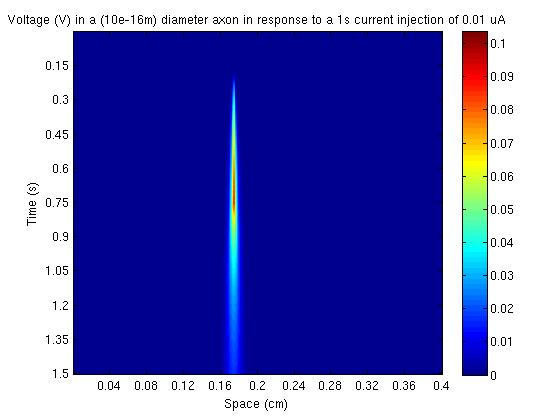
nlabels = 10;
xTick = [0:(Spacesteps/nlabels):Spacesteps];
yTick = [0:(Timesteps/nlabels):Timesteps];
xTickLabels = [0:Length/nlabels:Length];
yTickLabels = [0:T_max/nlabels:T_max];
clf;
imagesc(V);
set(gca, 'Xtick', xTick, 'XTickLabel',xTickLabels); xlabel('Space (cm)');
set(gca, 'Ytick', yTick, 'YTickLabel', yTickLabels); ylabel('Time (s)'); colorbar();
title(['Voltage (V) in a (10e-16m) diameter axon in response to a '  num2str(-1*(floor(T_max/8)-ceil(1*T_max/2)))  's current injection of ' num2str(-I_in) ' uA']);

% Set return variable
V_final = V;

end