1 Second Order Difference Kernels

1.1 Finite Difference Approximation

Based on Taylor approximations, finite difference approximations to the derivatives of a function defined on a uniform grid (x_i), x_i = x_o + h, h > 0 can be given using arbitrarily sized kernels. For second order kernels, we obtain the following ’forward difference’ approximation to the first derivative:

and a ’center difference’ approximation to the second derivative:

Note that these are not the only difference formulas that can be defined as computational molecules on the mesh; others such as backward or centered difference or the Crank-Nicolson molecule have various computational advantages related to ensuring stability while using differently spaced meshes.

1.2 Application to Cable Equation

The cable equation describes the passive spread of voltage in one dimension along a cable with an inner (’axial’) conductor and outer (’membrane’) resistive covering. The cable equation in a second order parabolic PDE, similar in form to the heat equation that describes the distribution of thermal energy along a uniform bar as a function of time and distance from the origin. The voltage in a cable as a function of time t and distance along the cable x can be given by

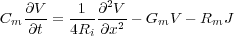
where C_m is the membrane capacitance; R_i is the longitudinal (internal) resistance; G_m is the membrane conductance (G_m = , where R_m is the membrane resitance); and J is the injected current.

If we let v_jⁿ = V (x_j,t_n), and partition time in steps Δt and space in steps Δx, we can use the second order difference approximations above to write the cable equation as

Rearranging terms so that the current terms at any grid step (v_jⁿ) can be expressed in terms of past values (v_j-jm^n-n_m) we obtain

Now we let K = and we let B = . Then we can write v_iⁿ⁺¹as:

We can write this in vector form if we take
vⁿ = (v_iⁿ) = ^t[..., v_i-1ⁿ , v_iⁿ , v_i+1ⁿ , ...]                            and
vⁿ⁺¹ = (v_iⁿ⁺¹) = ^t[..., v_i-1ⁿ⁺¹ , v_iⁿ⁺¹ , v_i+1ⁿ⁺¹ , ...]                      and
jⁿ = (J_iⁿ) = ^t[..., J_i-1ⁿ , J_iⁿ , J_i+1ⁿ , ...]


Then we have

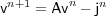
where A is defined as

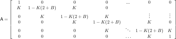
Thus, given a vector v⁰ specifying the intial condition, you can simply iterate forward in time, repeatedly applying the matrix A to the output of each previous step. Note that the top and bottom rows are set to 1 (identity) to preserve the boundary condition. In the simulations below, Dirichlet (fixed) boundary conditions are used, with the voltage fixed are resting potential (analagous to a sealed, but not killed, axon ending). A simple MATLAB function implementing this entire method is given in the file Cab7.m.

2 Fourth Order Difference Kernels

For fourth order kernels, following the conventions above we obtain the following finite difference approximations:

Note that the fourth order kernels are not symmetrical about x_i, which would lead to a linear decrease in the error (but not change its order), but the asymmetrical kernel is used to simplify the programming. Here we let K = and B = (-30 - 30K -) to yield the following matrix:

A =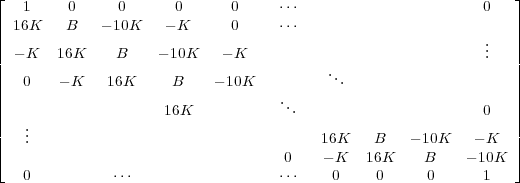

Then we can calculate the voltage vectors at each time step (as defined above) by:

3 Computational Issues

The requisite density of the mesh spacing is highly sensitive to the parameters K and B, particularly for the fourth order difference method. In practice, the mesh size required to ensure a stable solution to the cable equation with realistic biological parameters using the fourth order method is too fine to allow for simulation on a standard desktop computer due to memory restrictions. Thus, to approximate higher order differences, more efficient computational algorithms such as Crank-Nicolson or Runge-Kutta should be employed.

4 Results

4.1 Comparison with results from NEURON

The following figure shows the voltage trace at the current injection site computed using the parameters:

• R_m = 1 × 10³ Ω∕cm
• R_i = 35.4Ω ⋅ cm
• C_m = 1 × 10^-6 F∕cm²
• d = 1 × 10^-13cm   (again, this is smaller than in reality)
• T_max = .005s
• L = 0.01cm
• Δt = 1 × 10^-5s
• Δx = 2 × 10^-4cm

Figure 1: Voltage at the location of current input as a function of time as computed with the algorithm delineated in this report

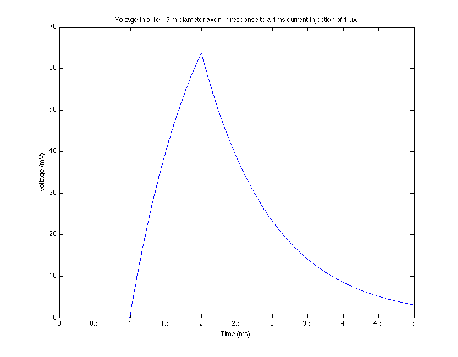
Running the simulation in the NEURON environment (see http://www.neuron.yale.edu/) with the same parameters yields the following voltage trace:

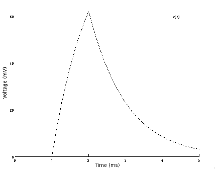
The similarity in shape (it is seen on further inspection that there are slight differences in amplitude) serves to validate the general approach outline above. However, the simulation of realistic biological parameters (similar to the default parameters given in NEURON) is computationally difficult for the reasons outlined above.

4.2 Visualizing current spread

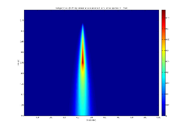
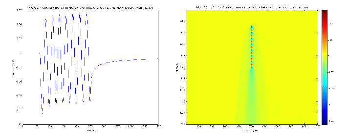
The solution to the cable equation was computed using the second order difference method with the following parameters:

• R_m = 2.5 × 10¹¹ Ω∕cm
• R_i = 29.7Ω ⋅ cm
• C_m = 1 × 10^-6 F∕cm²
• d = 1 × 10^-14cm   (this is smaller than in reality, but was used to allow a wider mesh space and thus allow the use of less memory)
• T_max = 1.5s
• L = 0.001cm
• Δt = 6 × 10^-4s
• Δx = 2 × 10^-6cm

A current injection of -0.01μA with a duration of 1 second was applied to the cable at a single location. The resulting voltage is shown below (Fig. 3) as a function of space and time.

4.3 Response to s sinusoidal current input

Using the same parameters as section 4.2 the voltage response to the input of a sine wave current amplitude was calculated. The results are shown in Fig. 4, which uses the same conventions as the figures above.

5 Discussion

The comparison of the numerical solution presented above with a model run in NEURON reveals that our method yields very reasonable results when run with parameters that fulfill criteria for stability. The dynamics of the voltage change in repose to current inputs match quite well. The figures also show a pattern of voltage spread that matches expectation based on experiment. Nevertheless, because differential equations are inherently functions of both the independent variables and the discrete step size in those variables (e.g. Δx), the computation of the solution using this method has some key limitations:

• Computational efficiency: Simulation of completely biologically realistic parameters required a mesh size too small to achieve a guarantee (or even possibility) of a stable solution. This can be predicted by the value of K in the second order case, which should be less than to ensure stability (likewise for B in the fourth order case – a condition that could not be met in useful simulations using the memory available on a desktop computer).
• Stability (oscillations): The computation introduces error into the solution that is guaranteed to be less than the O terms in the formula, but these errors may wax and wane periodically. Such behavior can be observed in the color map plots in the spatial (x) direction, where ripples are seen in regions that should be smoothly decreasing.

There are a number of other options for computing the difference approximations. One simple change that would improve the stability of the solution without changing the computational load would be to replace the forward difference approximation to the first derivative with a centered difference approximation, as in f′(x) ≃ + O(Δx²). In this case the error would only be proportional to the square of the time step (and thus would be reduced, since Δt < 1). Finally, as mentioned above, in many situations the use of more efficient and more stable algorithms (Runge-Kutta, Crank-Nicolson), which are in packages already widely available, would remedy the problems described here.

6 References

1. Christof Koch. Biophysics of Computation. Information Processing in Single Neurons. 1999. Oxford University Press.
2. http://reference.wolfram.com/mathematica/tutorial/NDSolvePDE.html#c:4
3. Gerald W. Recktenwald. Finite-Difference Approximations to the Heat Equation. http://web.cecs.pdx.edu/~gerry/class/ME448/codes/FDheat.pdf
4. Numerical Analysis of Partial Difference Equations. Hall and Porsching. 1990. Prentice Hall.
5. Numerical Solution of Partial Difference Equations: Finite Difference Methods 3rd ed. G.D. Smith. 1985. Oxford University Press.
6. NEURON for empirically-based simulations of neurons and networks of neurons. http://www.neuron.yale.edu/neuron